Anomaly Detective: a tool to quantify anomalies in time-series data

Click here to test the app!

Anomaly detection in time-series data is a long-standing problem in analytics, with wide range of applications in practice. Over many years, I got involved in solving different types of business problems where I collected and/or analyzed time-series data. In many cases, I performed feature engineering as well as built predictive models using data with a defined time axis. Regardless of the application, anomalies or outliers in time-series data can have profound impact on the resulting analysis and its applications.

There are many methods that can be used to detect anomalies in time-series data, ranging in their complexity. These approaches include application of simple heuristics, linear models, as well as elaborate machine learning algorithms. While practicing my work over the course of multiple projects, I realized simpler approaches tend to be more cost-effective in diagnosis of time-series anomalizes. This is because complex machine learning algorithms often require larger amounts of data to train, multiple parameters to estimate, and in many cases multiple hyperparameters to tune.

Over several years, I tend to use 2 main approaches to spot anomalies in my time-series projects. The first approach leverages z-scores after some decomposition, whereas the second approach involves fitting a model to quantify and infer anomalies. I streamlined these approaches into utilities to use them again and again for various projects and also built the Anomaly Detective , a web-based application that can automate anomaly detection process.

Here I describe this practical tool, as well as the two common methods you can use to detect anomalies in time-series data. The tool currently works for univatiate time-series, while I plan to expand its utility for multivariate series in near future. Simply upload your time-series as a single column csv file, choose the correct frequency of your data (e.g: Monthly), choose the start date of your series from the calendar and click "Monitor anomalies". The results of time-series anomaly detection will be presented in visualizations in a two-tab layout, each tab focusing on one of the detection method as I discussed below. You can interact with the plots by hovering individual data points, which would be enlarged depending on the severity of the anomalies deemed by a particular approach.

Z-scores to quantify time-series anomalies after STL decomposition

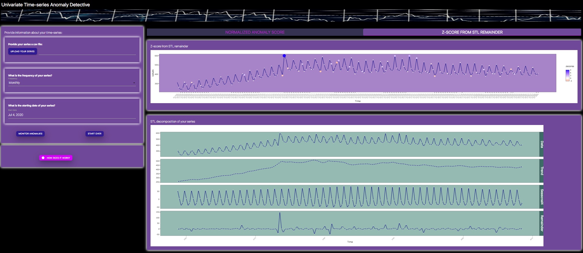
This is by far one of the simplest and most intuitive approach for identifying anomalies in time-series data. The approach essentially relies on the Seasonal and Trend decomposition using Loess (STL) process, particularly the 'remainder' from the STL decomposition. We can simply calculate z-scores using the remainder series and can monitor extreme values of these z-scores across the time axis. The approch provides a convenient way of identifying anomalies in the time-series data, after accounting for trend and seasonal components of the time-series data.

Despite the simplicity of this detection approach, there are a few caveats as well. First, interpretation of extreme z-scores assumes a Gaussian distribution, while many time series could be skewed. Second, this approach could be relatively sensitive, hence may highlight many data points as potential outliers.

Normalized Anomaly Scoring Algorithm

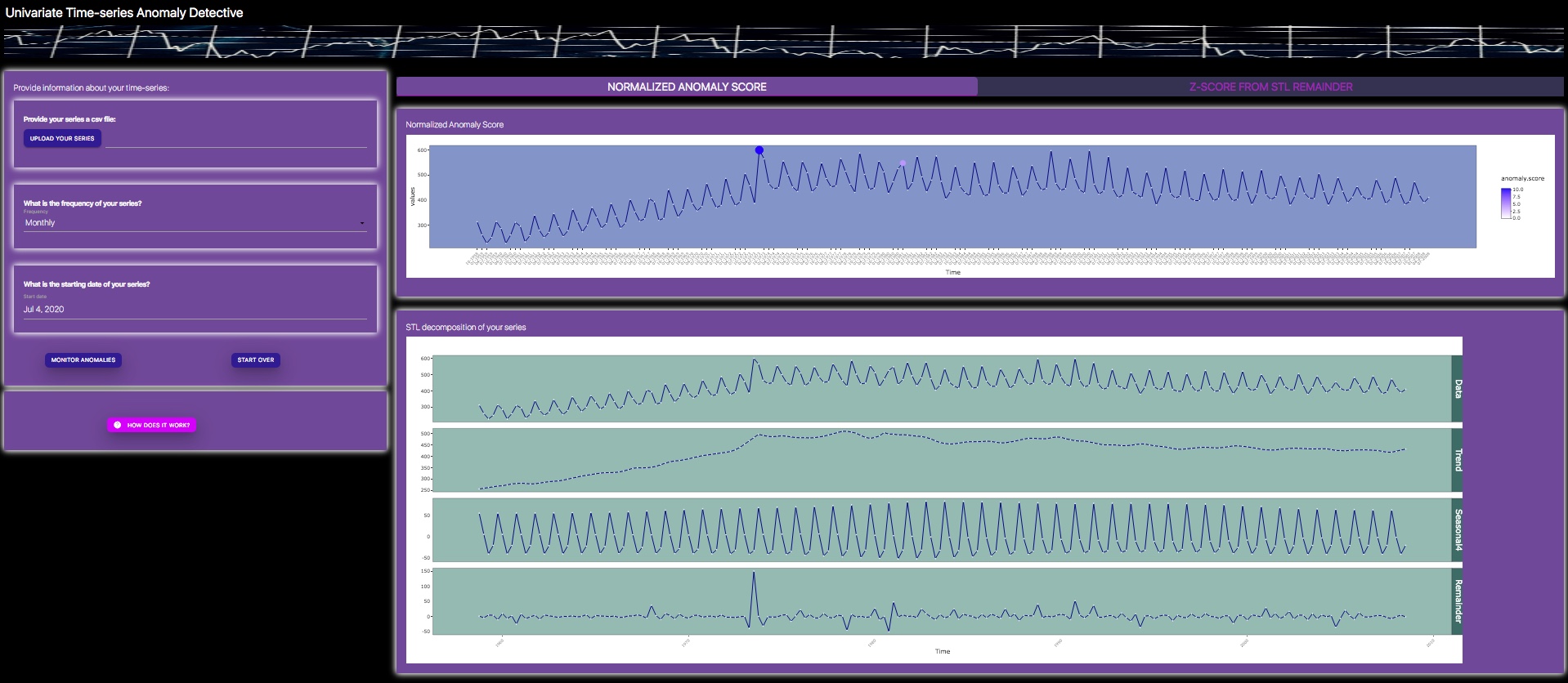
Given the potential caveats of using z-scores for anomaly detection, I wrote up a complementary algorithm that applies a 3-step process to identify potential anomalies in time-series data.

Identify: potential anomalies

• 1. Check if there is strong seasonal component, seasonally adjust data if necessary (more precisely if the variance of detrended data is higher than variance of robust STL remainder, by a fixed threshold).
• 2. Fit Friedman's Super Smoother (Friedman, 1984) to the resulting time-series.
• 3. Obtain residuals between the time-series and the data fitted on the smoothed line.
• 4. Infer outliers based on residuals that are outside of the interquartile range.

Suggest: a replacement

• 5. Assume the identified outliers as "Missing Data at Random"(note that this may or may not be a correct assumption for any given outlier).
• 6. Perform linear interpolation to calculate potential replacement(s) for outlier(s): fit a polynomial linear regression and Fourier transformation to build an imputation model to predict missing values. Note that if there is seasonal component, we first seasonally adjust using robust STL, then perform linear interpolation to seasonally adjusted series. We then add back the seasonal component if any.

Finalize: anomaly score standardization

• 7. Calculate the difference between any outlier and its suggested replacement.
• 8. Normalize this difference to standard deviation of the "remainder" from robust STL of entire time-series.

Final words:

I hope you enjoyed learning about this tool. Feel free to use the app for your own anomaly detection problems when dealing with time-series data!